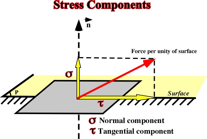
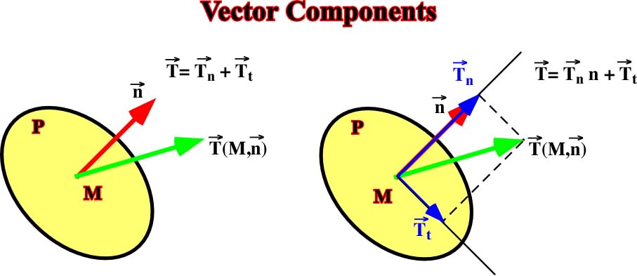
Fig. 1- Normal and shearing components of a stress applied on a surface

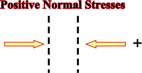
Fig. 2- Compressional or positive normal stresses are generally depicted by convergent arrows or by a symbol plus

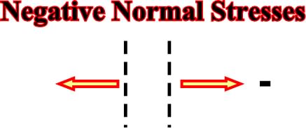
Fig. 3- Tensional or negative normal stresses, acting in a plane, are represented by two arrows in opposite directions or by the symbol minus.

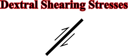
Fig. 4- Very often, dextral shearing stresses are represented, as dextral fault, by two opposite arrows, one above and the other below the plane, indicating that the upper part is displaced to the right.

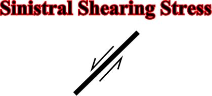
Fig. 5- Sinistral shearing stresses are represented, as sinistral fault, by two opposite arrows, one above and the other below the plane, indicating that the upper part is displaced to the left.

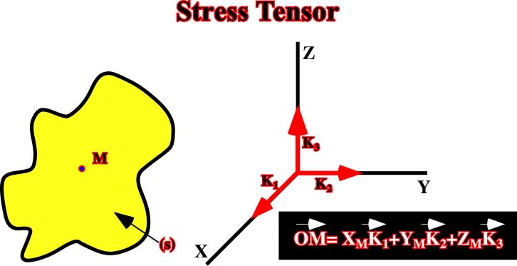
Fig. 6- The arbitrary point M can be defined by three orthogonal coordinates, where K1, K2 and K3 are unitary vectors.

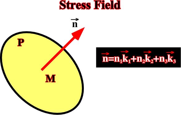
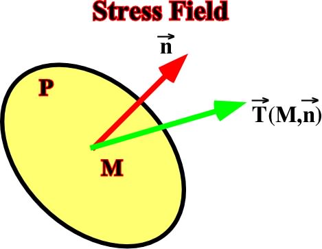
Fig. 7- The stress field for the point M is defined by the vector T= (M,n)

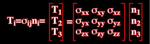
Fig. 8 - The stress vector (T) can be represented by three components T=(M,n), and (M+n) = T1 k1 + T2 k2 + T3 k3.

The relations between (T1,T2,T3) and (n1, n2, n3)

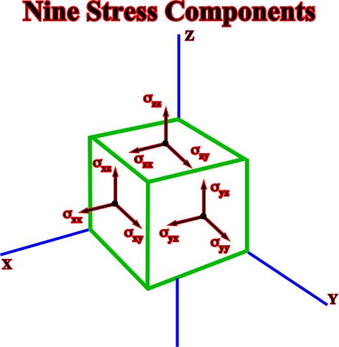
Fig. 9- Stress components can be illustrated graphically. All elements, that is to say, vector, point, body, etc., are referred to the coordinate axes (x,y,z), which origin is O.

Fig. 10- In this figure, Tn is the normal stress and Tt the tangential or shearing stress. Conventionally, when Tn is positive, normally, there is compression, when Tn is negative there is extension

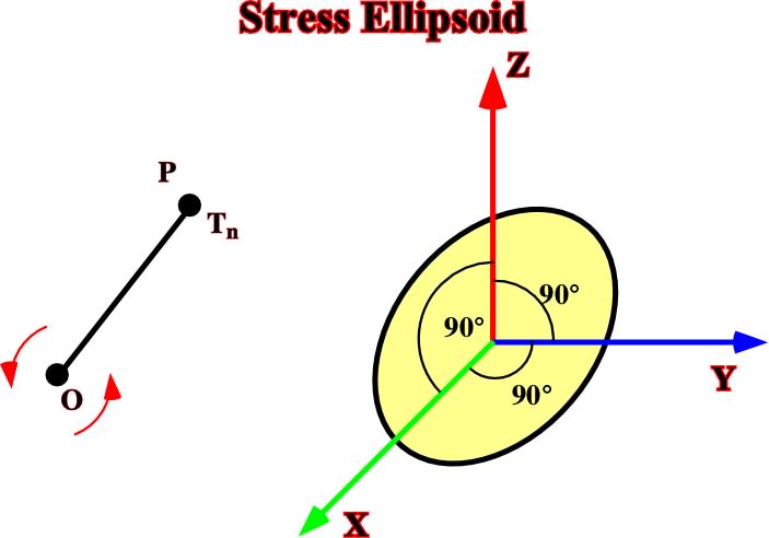
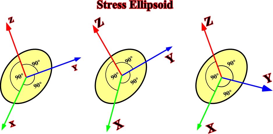
Fig. 11- Stress ellipsoid creating by rotation of vector (n) in all direction. Such ellipsoid is characterized by the following equation: xxX2+yyY2+zzZ2+2xyXY+2yzxYZ+2zxZX

Fig. 12- Changing of coordinates does change the stress ellipsoid.

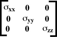
The tensor

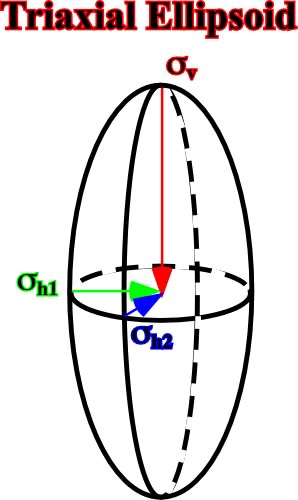
Fig. 13- In a triaxial ellipsoid, the three principal axes are different. v is the vertical stress, while h1 and h2 are the horizontal stresses. Note that along these axes there are no shearing stresses

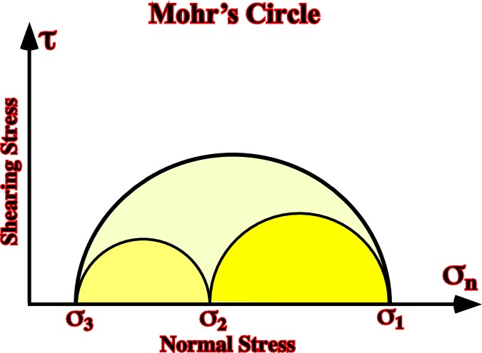
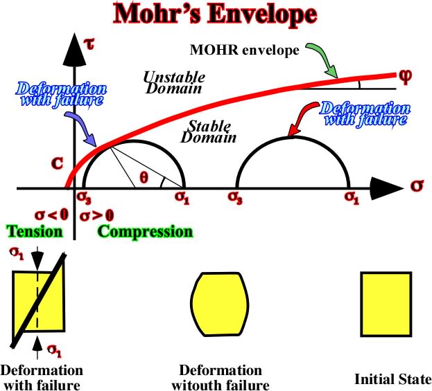
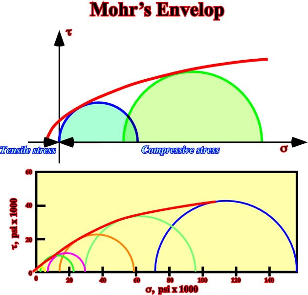
Fig. 14- The Mohr�s circle is a graphic representation of the state of stress at a given point at a given time. The coordinates of each point on the circle are the shear stress and the normal stress on the given plane. The Mohr envelope (fig. 52) is an envelope of a series of Mohr circles, that is to say, the locus of points whose coordinates represent the stresses at failure.

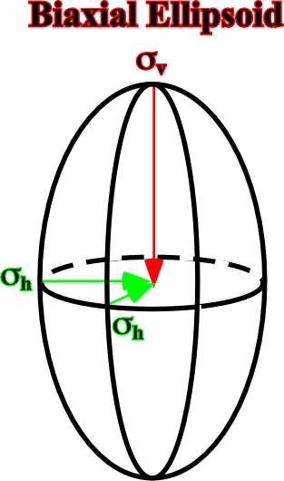
Fig. 15- In a biaxial ellipsoid there are only two principal axes. The vertical axis (v) and the horizontal axis (h). In other words the equatorial plane of the ellipsoid is a circle.

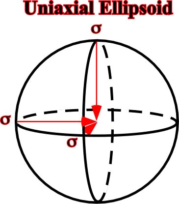
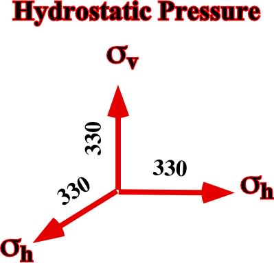
Fig. 16- In an uniaxial ellipsoid the stress stays constant independently of its orientation. The ellipsoid has the shape of a circle and its radius is . A typical example of uniaxial ellipsoid is the hydrostatic pressure, i.e. the pressure of liquids.

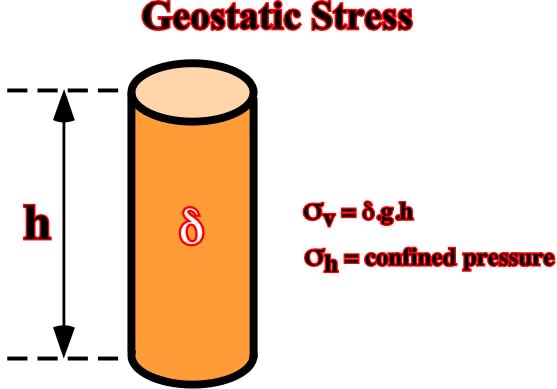
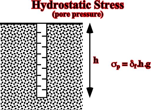
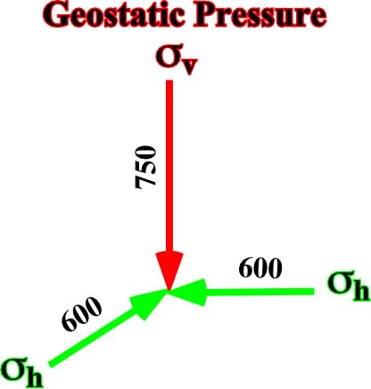
Fig. 17- The hydrostatic stress can be depicted by a biaxial ellipsoid, in which the sv is the weight of the sedimentary column (d.h.g) and the h the confined pressure (6-8/10 of v). The average density of the sedimentary colum is d , h is the height of the column and g the gravitational force.

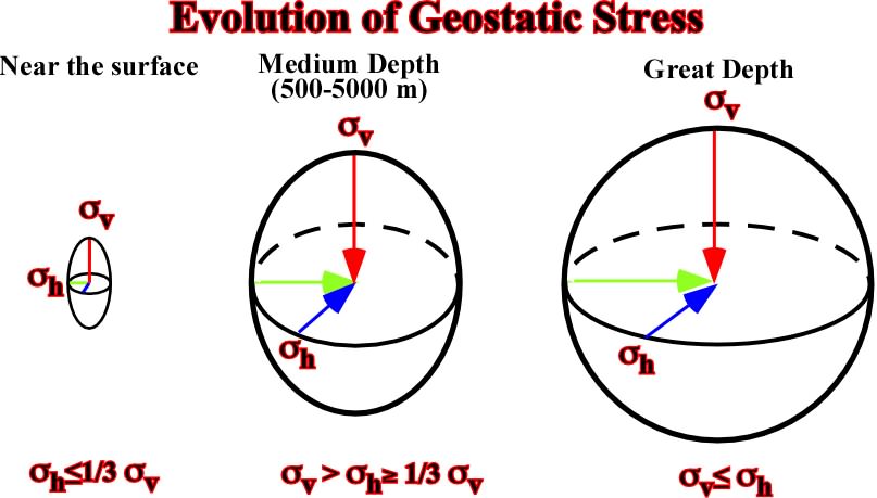
Fig. 18- This figure illustrates the evolution in depth of the geostatic stress. Near the surface, the ellipsoid is biaxial and oblong, but in depth becomes almost uniaxial. Such a feature explains, partially, why fault planes flatten in depth.

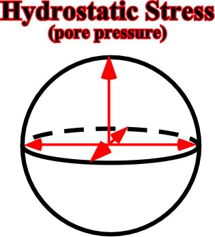
Fig. 19- At a given depth, the pore pressure can be represented by a uniaxial ellipsoid, that is to say, a sphere, which radius is the product of the density of the fluid (df). The depth of the given point is (h) and the gravitational force is (g).

Fig. 20- Pore or hydrostatic pressure acts in opposite direction of the lithostatic pressure. It explains buoyancy, that is to say, the upward thrust on a body immersed in a fluid. This force is equal to the weight of the fluid displaced (Archimedes� Principle).

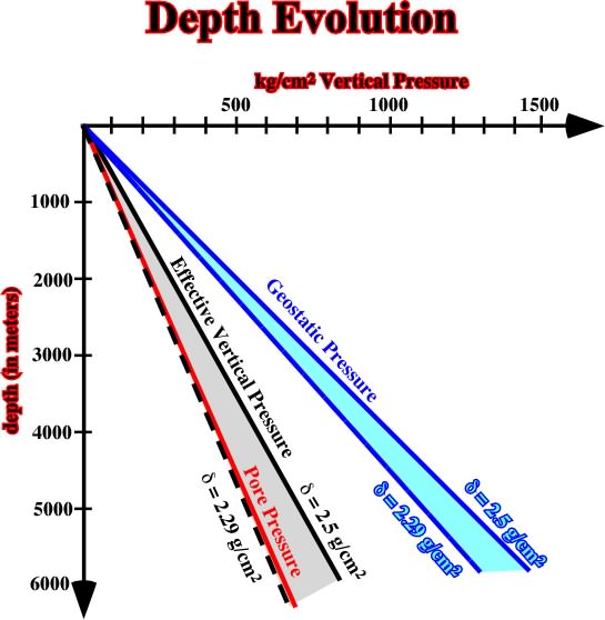
Fig. 21- This cross-plot represents the evolution, in depth, of the geostatic pressure, pore pressure and effective vertical pressure.

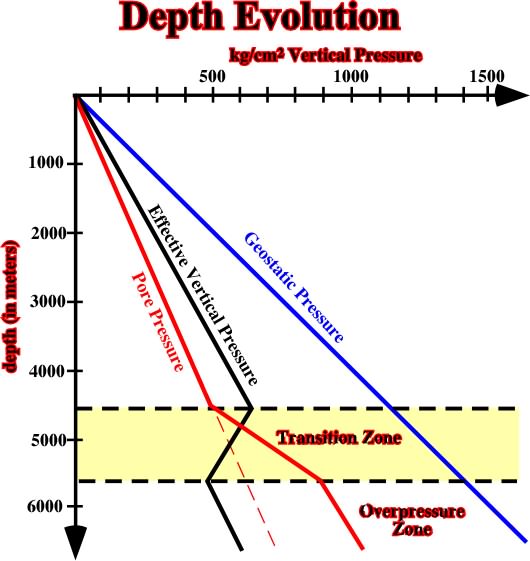
Fig. 22- This cross-plot illustrates the evolution, in depth, of vertical effective pressure in a basin with an overpressure zone.

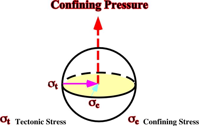
Fig. 23- When a tectonic stress is added in a given direction, it induces, by reaction, a lateral confined pressure. Upward (free surface) an equilibrium pressure is created whether by uplift or subsidence.

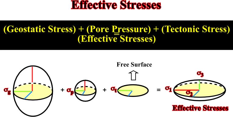
Fig. 24- The effective stresses (1, 2, 3), which are those that deform the sediments, correspond to the addition of the geostatic pressure, the pore pressure and the tectonic pressure.

Fig. 25- Principal axes of the ellipsoid representing the geostatic pressure g.

Fig. 26- Principal axes of the ellipsoid representing the hydrostatic pressure p.

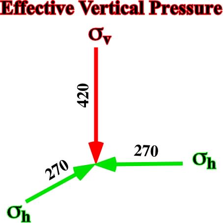
Fig. 27- Principal axes of the ellipsoid representing the effective vertical pressure ev.

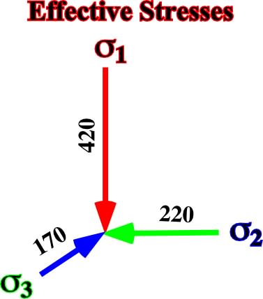
Fig. 28- Principal axes of the ellipsoid of effective stresses after adding a tectonic stress of -100 kg/cm2 (horizontal tension) along the axis Y (blue) of a bidimensional vertical effective stress with v=420 kg/cm2 and a h= 420 kg/cm2.

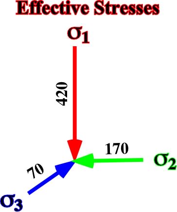
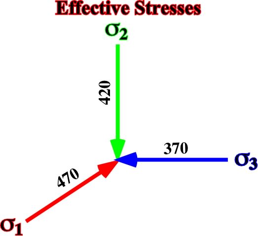
Fig. 29- Principal axes of the ellipsoid of effective stresses after adding a tectonic stress of -200 kg/cm2 (horizontal tension) along the axis Y of a bi-dimensional vertical effective stress with v =420 kg/cm2 and a h =420 kg/cm2.

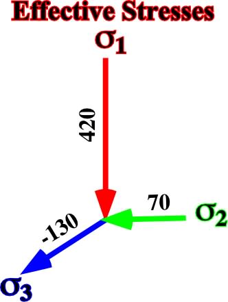
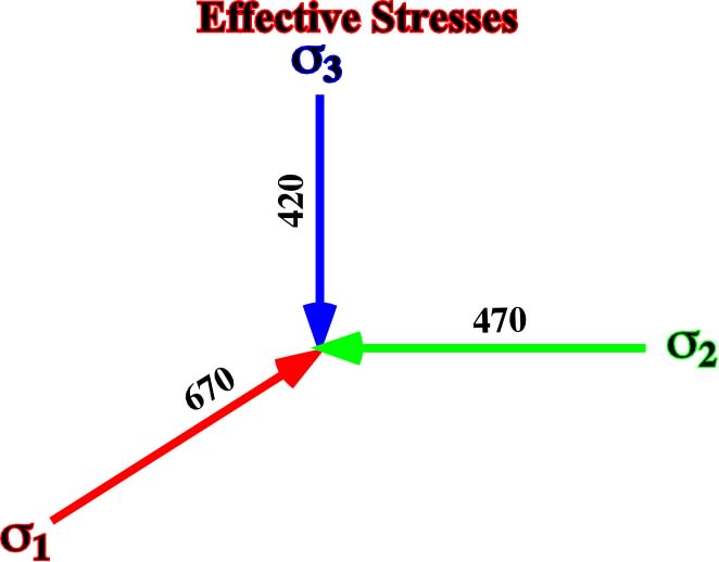
Fig. 30- Principal axes of the ellipsoid of effective stresses after adding a tectonic stress of -400 kg/cm2 (horizontal tension) along the axis Y of a bi-dimensional vertical effective stress with v =420 kg/cm2 and a h =420 kg/cm2.

Fig. 32- Principal axes of the ellipsoid of effective stresses after adding a tectonic stress of 200 kg/cm2 (horizontal compression) along the axis Y of a bidimensional vertical effective stress with v =420 kg/cm2 and a h = 420 kg/cm2.

Fig. 33- Principal axes of the ellipsoid of effective stresses after adding a tectonic stress of 400 kg/cm2 (horizontal compression) along the axis Y of a bidimensional vertical effective stress with v =420 kg/cm2 and a h = 420 kg/cm2.

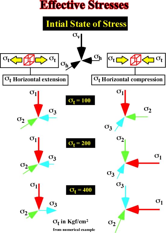
Fig. 34- This sketch summarize all possible ellipsoids of effective stresses (1, 2,3) when adding a negative (extension) and a positive (compression) tectonic stress (t) an initial state of stresses (v, h). When 1 is vertical, the sediments are lengthened by normal faults striking parallel to 2. When 1is horizontal, the sediments are compressed by folds or reverse faults striking parallel to the medium effective stress, that is to say, 2.

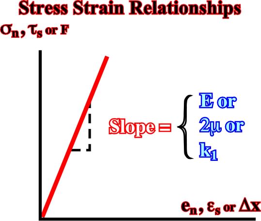
Fig. 35- The stress-strain relationships in a linear elastic (Hookean) solid (or a spring) are here illustrated by a plot of normal stress (or force) versus extension, where the slope E (or k1) is the Young�s modulus (or spring constant).

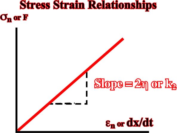
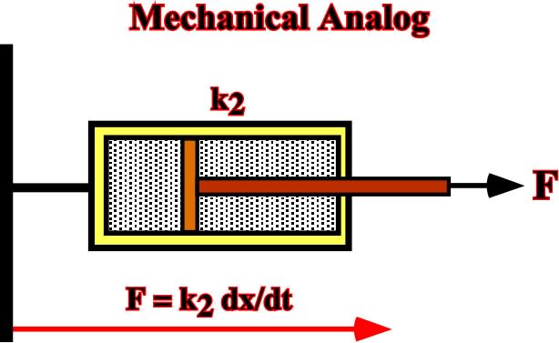
Fig. 36- The characteristics of a linear viscous fluid (or Newtonian) are here illustrated by the plot of stress (or force) versus incremental strain rate (or displacement rate). This plot has a slope h (or k2, dashpot)), that is to say the coefficient of viscosity (dashpot constant k2

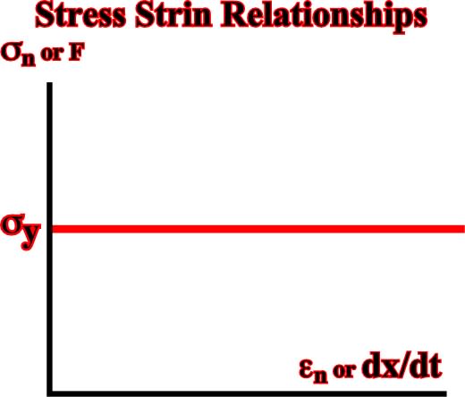
Fig. 37- This figure illustrates the characteristics of a perfectly plastic (Saint Venant) material on a plot of stress (or force) versus incremental strain rate (or velocity).

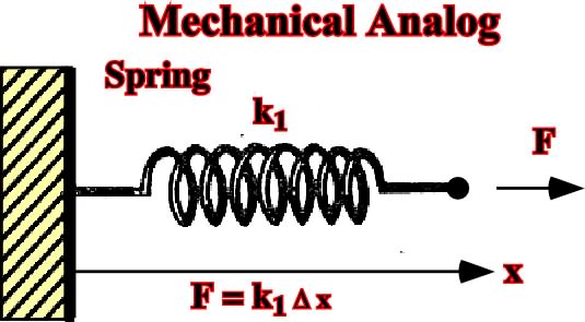
Fig. 38- A mechanical analogue to elastic behavior (strain is proportional to stress) consists of a spring with spring constant k1 attached to a rigid wall, subjected t a force F, and displaced a distance Dx beyond its unloaded length.

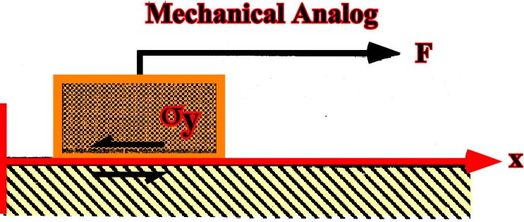
Fig. 39- A plastic solid behavior (strain starts when shearing exceeds a threshold) can be depicted by a body over a planar surface displaced by a rope. Once sliding has started, the applied force cannot rise above the frictional resistance regardless of the velocity of sliding, except during acceleration. Thus the force history produces an undefined rate of displacement.

Fig. 40- The analog of viscous behavior (Newton liquid) is tin a dashpot consisting of a porous piston in a cylinder containing a viscous fluid, attached to a rigid support, and subjected to a force F.

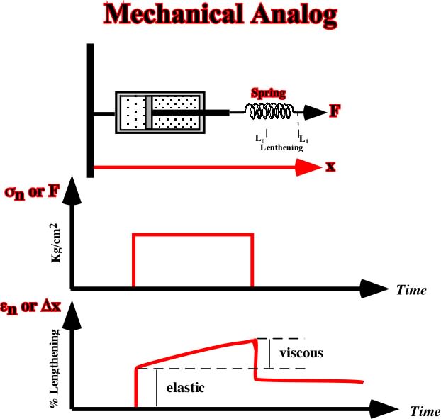
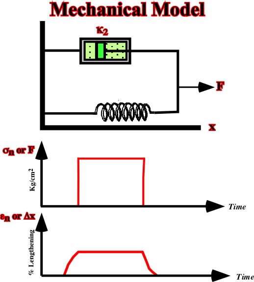
Fig. 41- The characteristics of a visco-elastic, or Maxwell, material are here illustrated by a mechanical analogue consisting of a dashpot in series with a spring. The plot sn or F versus time shows the stress-time history imposed on the material, while the plot en or Dx indicates the natural strain-time response to the imposed stress, which includes an instantaneous recoverable elastic deformation and a non recoverable viscous deformation.

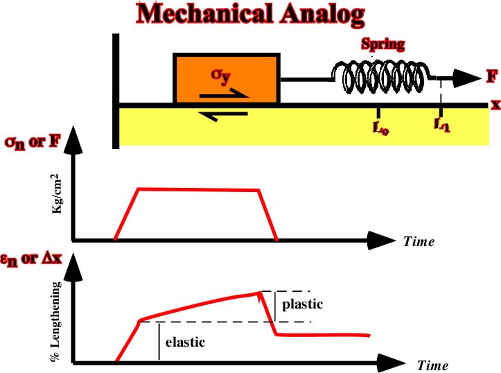
Fig. 42- The mechanical analogue for an elastico-plastic material (or Prandtl) consists of a friction block connected in a series with a spring. An imposed stress-time history and the corresponding natural strain-stress history are also illustrated. Below the yield stress, the material deforms elastically. At the yield stress, plastic deformation occurs at undetermined rate. When stress is removed, the elastic portion of the strain recovers, leaving a permanent strain equal to the plastic portion.

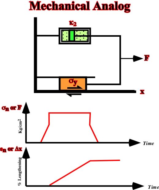
Fig. 43- Here are illustrated the characteristics of a visco-plastic, or Bingham material. The mechanical analogue consists of a dashpot and a friction block connected in parallel. A stress-time history and the subsequent natural-strain-time history resulting from the imposed stress are also depicted.

Fig. 44- The mechanical analogue of a firmo-viscous behavior consists of a dashpot and a spring connected in parallel as illustrated. The natural strain-time response of an imposed stress-time history shows that the incremental strain rate depends both on the initial stress and on the strain.

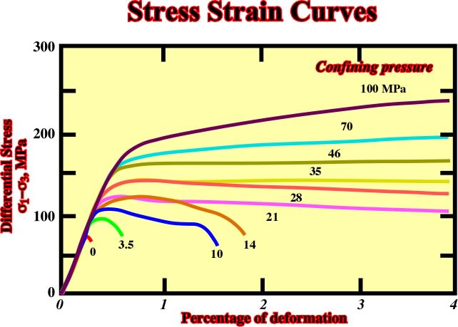
Fig. 45- Progression of stress-strain curves with increasing of confining pressure in the Wombeyan marble (from Paterson, 1978).

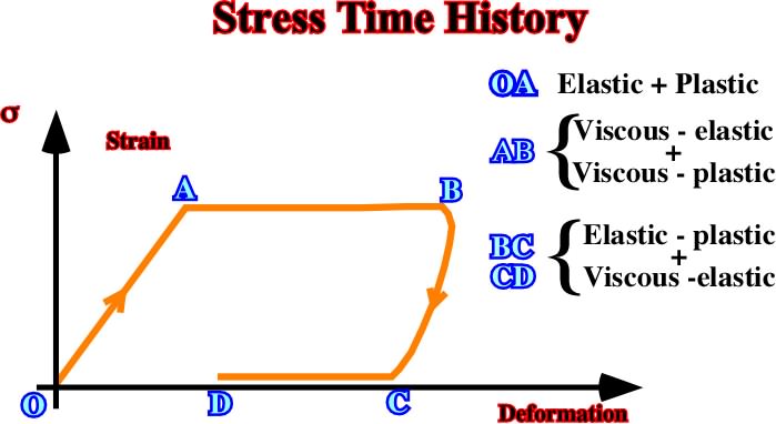
Fig. 46 �In this example, the stress-time history and the associated natural stress-time response are shown. The behavior is elastic-plastic during OA, then during AB it comes visco-elastic / viscous-plastic, and finally, between BC and CD it is Elastic-plastic / visco-elastic.

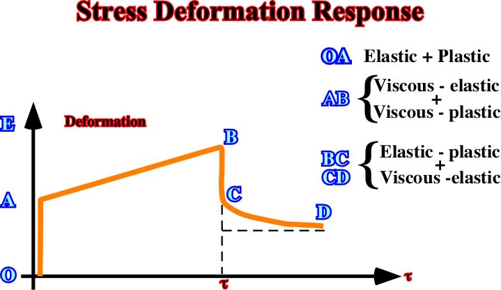
Fig. 47- In this stress-deformation response, during OA the material behavior is elastic-plastic, during AB it behaves as visco-elastic / visco-plastic, while from B to C and D, it behaves as elastic-plastic / visco-elastic.

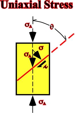
Fig. 49- An uniaxial stress A is solved in a normal stress and a shearing t on the failure plane.

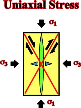
Fig. 50- Model showing the relationships between the three kinds of fractures in a rock under a uniaxial stress.

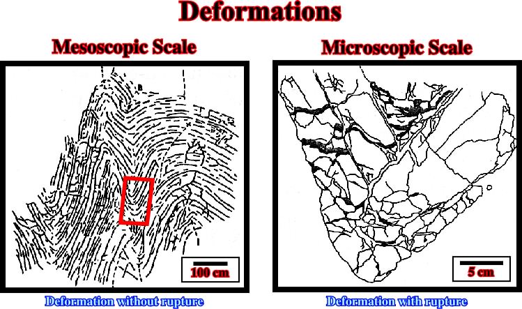
Fig. 48- At mesoscopic scale (scale of a continuous outcrop) deformation can be considered as without rupture, while a close-up of the outcrop (microscopic scale) exhibits deformation with rupture (from A. Droxler, 1982). On other hand, it is interesting to note than at mesoscopic scale, the deformation looks homogeneous, but at microscopic scale, dissolution (areas in black) clear indicates that its is not.

Fig. 52- The Mohr�s envelope intersects the shearing axis t at a value C called the cohesion of the material, which must be overcome priori to the development of a fracture plane.

Fig. 53- Example of a Mohr�s envelop in an Hauterivian limestone. Note than failure is easier under tensile stresses than compressional stresses

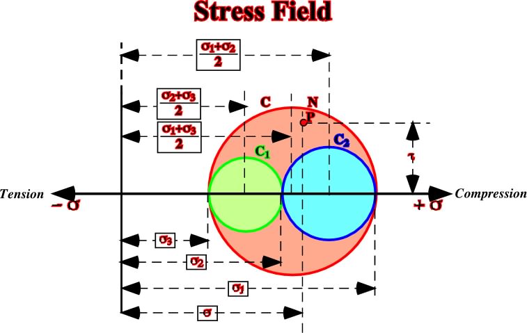
Fig. 51- Representation of the Mohr�s circle in three dimensions.

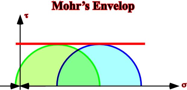
Fig. 54- Shaly sediments are so deformed than their pore-fluid cannot escape. Under these conditions, the Mohr�s envelop is a line parallel to the abscissa coordinate and its value is the tangential stress t.

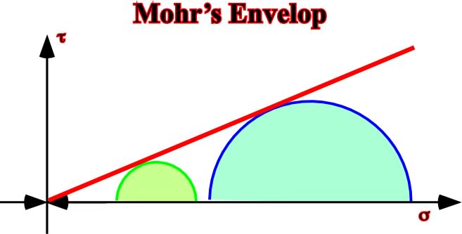
Fig. 55- As in this example the Mohr�s envelop intersects the shearing axis (ordinate) at a 0 value to t, i.e, that (= t), the material as not cohesion; it can resist to non-tensile stress.

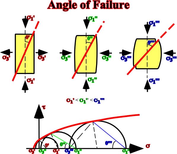
Fig. 56- The evolution of the failure angle explains why the angle of the faults planes increases in depth, that is to say, that the fault planes flattened in depth.

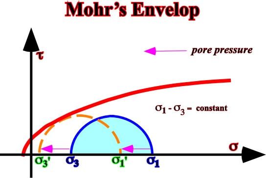
Fig. 57- Detachement planes, slopes failures and slumps, etc., can be explained by an increasing of the pore pressure.

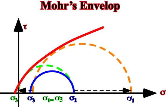
Fig. 58- This Mohr�s envelope illustrates the increasing of the confining pressure, which induces the stress-failure.

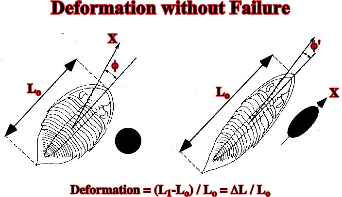
Fig. 60- Deformation without failure. The elongation can be calculate as (L1-Lo) / Lo.

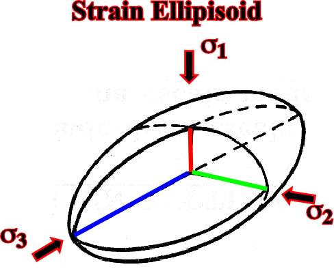
Fig. 61- In a strain ellipsoid, the direction of the maximum extension corresponds to the direction of the maximum effective stress, while the direction of the maximum shortening corresponds to the direction of the minimum effective stress, that is to say, 3.

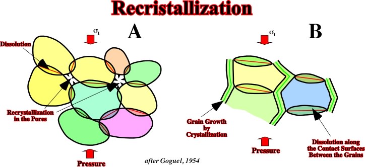
Fig. 62- Model proposed by Goguel explaining recrystallization in pore spaces

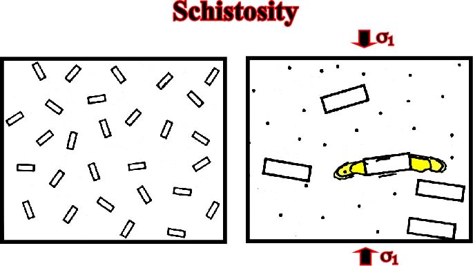
Fig. 63- The schistosity is in relation with the elongation and stretching of the rocks, that is to say, with the lengthening and mineral recrystallization along a particular direction.

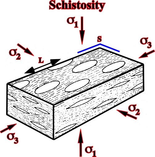
Fig. 64- The schistosity plane (s3, s2) is developed perpendicular to the maximum effective stress, that is to say, 1, on which one can recognize a lineation L oriented along the 3, i.e. perpendicular to the medium effective stress.

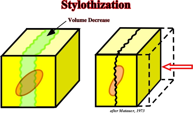
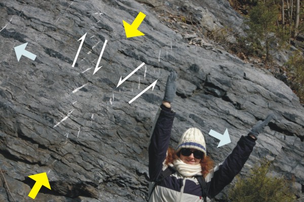
Fig. 65- Styloliths are a consequence of mineral dissolution perpendicular to the maximum effective stress

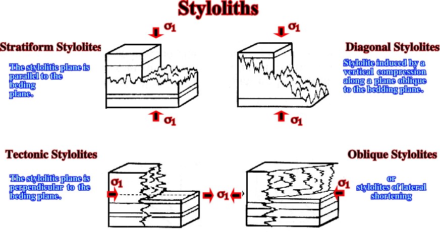
Fig. 66- Different type of styloliths associated with the maximum effective stress, 1.

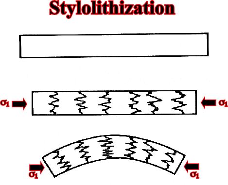
Fig. 67- Stylolithization that appears in the onset of deformation.