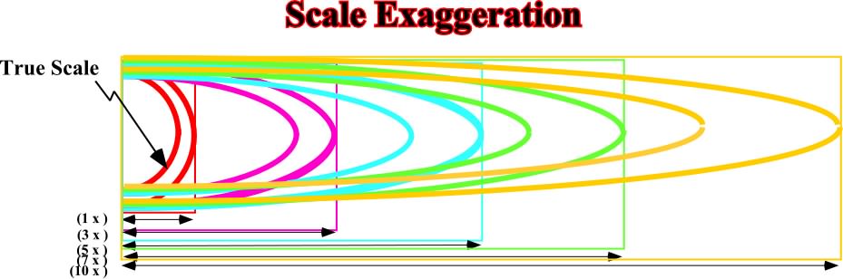
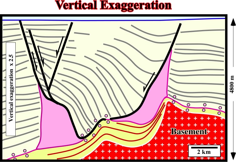
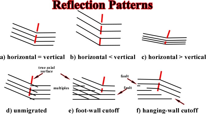
Fig. 85- Effects of vertical exaggeration on stratigraphic thickness and dips on beds of a unit thickness anticline anticline (from Sitter, 1974).

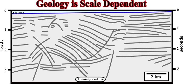
Fig. 86- Seismic lines are roughly time profiles. So, when interpreted, in geological terms, interpreters should not forget that Geology is scale dependent. In other words, interpreters must take into account not only the horizontal and vertical scales but lateral velocity changes as well. In addition, when working with unmigrated seismic data, as seismic horizons (chronostratigraphic lines) are not in its real position, the geometry and internal configuration of seismic interval must be carefully determined.

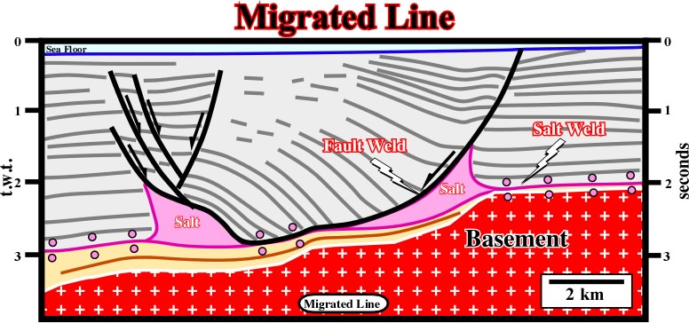
Fig. 87- The migrated version of the previous line, in spite of the fact that vertical scale is in time, has the appearance of a cross-section. The large majority of the diffractions has disappear. However, the seismic reflections are not in their really position and the lateral changes of velocity is not apparent. Therefore, the interval thicknesses and the dip are the reflections is apparent (compare with fig. 88).

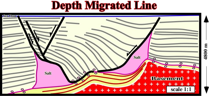
Fig. 88- On This seismic line lateral changes of the velocity induced either by thickness'' variation of the evaporitic layer (high velocity) and/or the Tertiary depocenter (low velocity) are not adequately corrected. The bottom of the salt layer (or salt weld) should not be undulated but planar.

Fig. 89- On this vertically exaggerated version of the line illustrated on fig. 88, it is quite evident the undulations (seismic pitfall) of the bottom of the salt are too exaggerated. Similarly, the dips of the normal faults (stretching faults), associated with the apex of the antiform, are higher than predicted by Anderson''s law. The same happens with the fault weld bordering the depocenter. It is interesting to notice the fault weld is underline by a seismic reflector. In fact, the fault gauge zone, is filled by salt, which creates a strong positive acoustical impedance contrast with the low-velocity sediments of the depocenter.

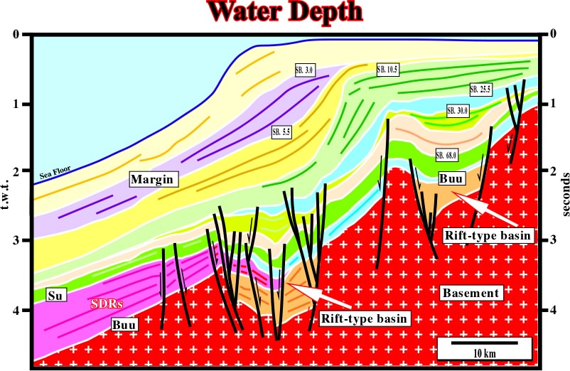
Fig. 90- On this line (western offshore India), due to the abrupt changing in water-depth (limit between the platform and upper continental slope) and, also, to the continuous seaward water-depth increasing, the apparent geometry of the reflectors is deformed. In fact, the seaward dip of the subaerial lava flows (SDRs, i.e. seaward dipping reflectors) is quite exaggerated, since the velocity of the seismic waves in the water is much lower than in sediments. Indeed, very often, in the distal areas of continental divergent margins (e.g. offshore Angola or Brazil), the geometry of the reflectors can be inversed; on a time seismic, the sediments dip seaward, but in time-depth conversion version, they dip landwards.

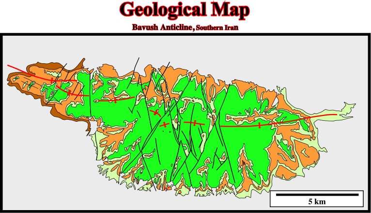
Fig. 91- The elongation the Bavush anticline (onshore Iran) along the 2 is quite evident on this geological map. The vertical conjugated faults, which elongate it, show clear horizontal slickensides, therefore they are strike-slip faults and not normal faults. In other words, as said previous, during a compressional tectonic regime, it is impossible to develop normal faults in the apexes of anticlines (sediments cannot be shortened and lengthened at same time in same place). However, very often, seismic interpreters, wrongly, consider such a strike-slip faults as normal faults.

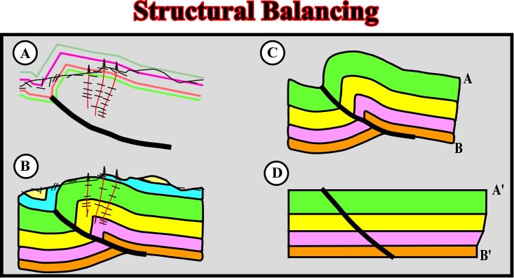
Fig. 92- Structural interpretations must respect the Goguel''s law, they must be equilibrated, that is to say, the volume of sediments must be kept constant during deformation. So, in this particularly example, in which a geological cross-section was built using well-dipmeter results, the geometry of the reverse fault is paramount. Indeed, when unfolding the sediments, they must be displaced along the fault plan without creating voids (missing sediments) or overlapping (too much sediments).

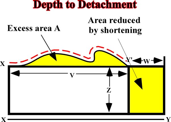
Fig. 93- Admittedly, in order to respect Goguel''s law, the area A (excess area) must be equal to the area B (area reduced by shortening). Knowing the area A and the horizontal shortening W, which can easily be determined (W=XY-V), it is possible to determine the dйcollement depth Z. Indeed, Z =(area A)/W, since area A = Area B = WZ.

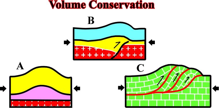
Fig. 94- In A, volume conservation is realized by folding and dйcollement on an underlying mobile layer (salt or shales). In B, volume conservation is realized by folding and faulted or imbricated basement; the pre-existent normal fault is reactivated, as reverse fault, during the compressional tectonic regime. Finally another way to respect the Goguel''s law is imbrications, which generally develops in uniform competent sediments such as limestone''s.

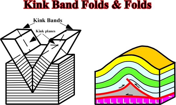
Fig. 95- The basal space problem of d�collement kink bands can be explained by the importance of the mobile layer thickness. It may be schematically assumed that its compression is achieved by means of the elimination masses used to fill the basal triangular space of kink bands.

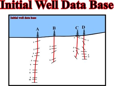
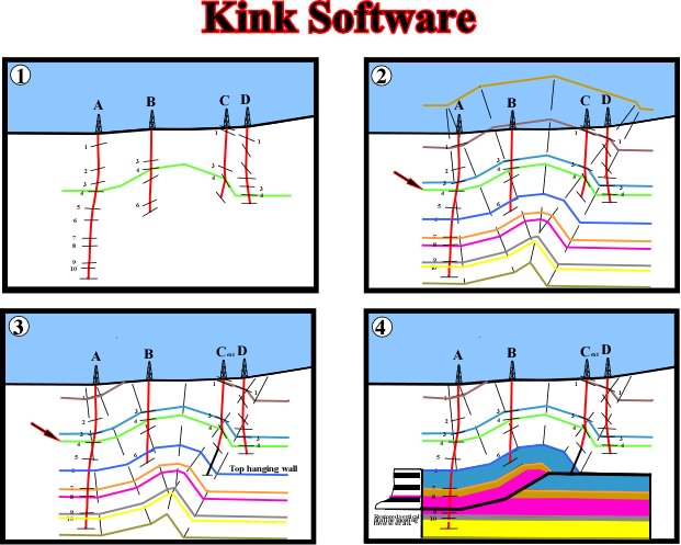
Fig. 96- The initial data base is given by the interpretation of the dipmeters logs and the stratigraphy of four wells. The profile A, B, C, D is perpendicular to the strike of the beds, so, the they are real dips.

Fig. 97- Using dip projections an horizon is constructed through the top of 4 formation compatible with all dip information (step 1), then its geometry is projected above and below the constructed 4 top horizon to check data compatibility(2) and extended until the top of the hanging wall is located (2). Now the section can be quickly modified by projecting the detachment plane and leading thrust fault surface and by constructing the horse and its internal geometry (3); The horse is restored to examine the state of strain in the sheet (4).

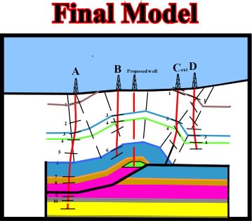
Fig.98- Finally, a complete new model with predicted horse is established, which implies a new strategy, that is to say, drill through top of predicted anticline to top of oil potential trap.

ig. 99- In this model, the faults of the upthrown block die on a detachment plane. When an interpretation of this kind is proposed, geologist must be sure than volume problems are respected.

Fig. 100- This model, quite similar to the previous one, require to be strongly critised when proposed in a geological interpretation, particularly of a seismic line.

Fig. 101- When migrated seismic lines were not available, this method was quite usefull. Presently, as the large majority of the seismic lines are migrated, it becames obselet.

EXTENSION: Fig.102- As during deformation the volume of sediments must be kept constant (no voids, or overlapping), in a cross-section oriented perpendicularly to the transportation axis, the area A is equal to area B and area C. Thus, knowing the heave of the fault, h, one can accesses de depth of detachment, d, by d= area C/h.

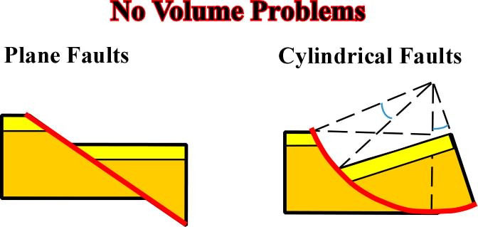
Extension:Normal Faulting Fig. 103- In a planar fault there is translation and both faulted blocks have the same dip, so there is not significant volume problems. Similarly, in a cylindrical fault, the rotation of the hangingwall induce a different dip from the footwall, but there is no major volume problem.

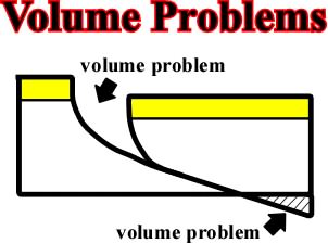
Extension, normal faults Fig. 104- In this example, without scale, a post-depositional extension creates two major problems: (i) a void and (ii) an overlapping. Subsequently, in order to respect Goguel''s law, sediments must accommodate to the new space conditions.

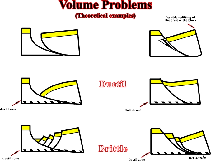
Extension, faulting -Fig. 105- These types of deformation are often observed when faulting becomes less active in a ductile layer within the sedimentary section (shale, salt, etc.).

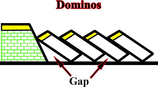
Extension:Fig. 106- Dominos are characterzed by no relative dip rotation between faulted blocks and by the fact that some mechanism is required to accommodate the space at the footand the end of the each block (gap).

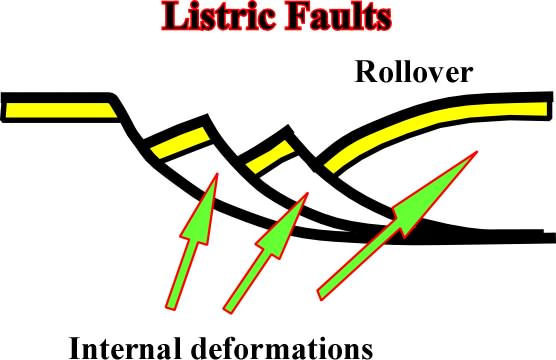
Extension: Fig. 107- A listric fault (from Greek "listron", i.e., "shovel") implies a rotation of the hangingwall, which controlled, or is controlled, by the depth of the detachment plane. As we will see next, the depth of the detachment can be predicted from the geometry of the rollover of a growth fault (fig. 108).

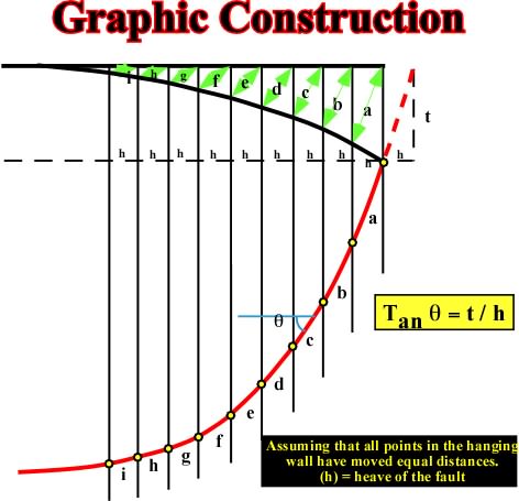
Fig. 108- Knowing: (i) the geometry of the hanging wall rollover, (ii) the heave (h) and assuming that it is the same for all points, (iii) the distance t, between each point of the rollover and the horizontal, one can calculate graphically the tan f as equivalent to t / h. Each value of tan f gives a, b, c, d, etc. The values a, b, c, d, e, etc., are then projected between the vertical of each considered point in the hanging wall, as illustrated hereunder.

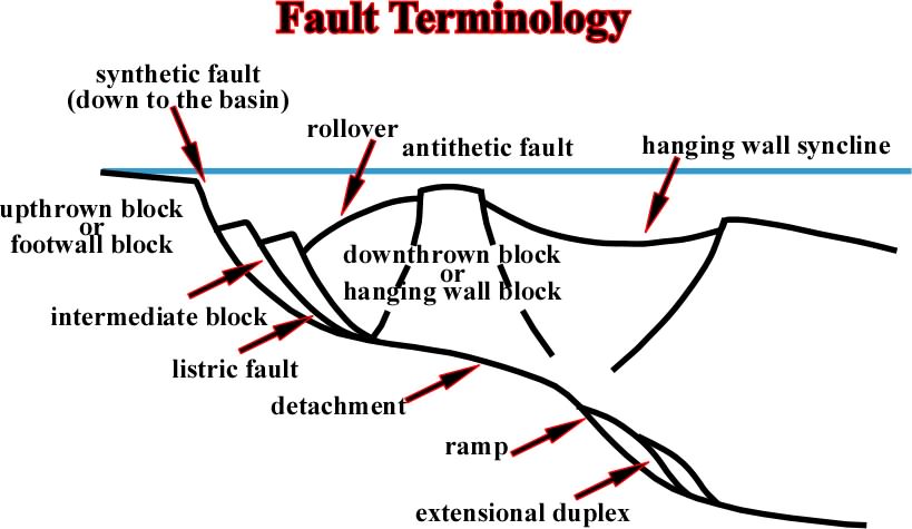
Fig. 109- In extensional tectonic regimes a esoteric jargon is often used, particularly by Anglo-Saxon geolgists. As depicted above the chiefly words are: (i) Synthetic faul, (ii) Upthrown bloc or footwall, (iii) Rollover, (iv) Anthitetic fault, (v) Hangingwall syncline, (vi) Downthrown block or hangingwall, (vii)Intermediate clock, (viii) Listric fault, (ix) Detachment, (x) Ramp, (xi) Extensional duplex, etc.

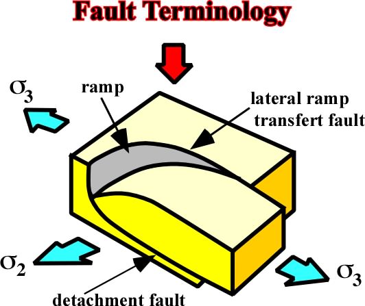
Fig. 110- A growth fault is a listric fault active during sedimentation and, generally, with a shallow detaching. The throw increases with depth and the strata of the downthrown side are thicker than the correlative strata of the upthrown side. A detachment plane, a ramp and a lateral ramp (or a transfert fault) are often used ti characterized part of a whole growth fault

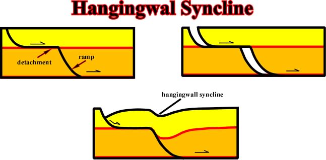
Fig. 111- As illustrated, it is evident that a hangingwal syncline is an extensional structure and not a compressional structure. It is associated to the lengthening of the hangingwall in order to respect the Goguel''s law. The displacement of the hangingwall creates potential voids and so the sediments must accommodate to the new volume conditions.

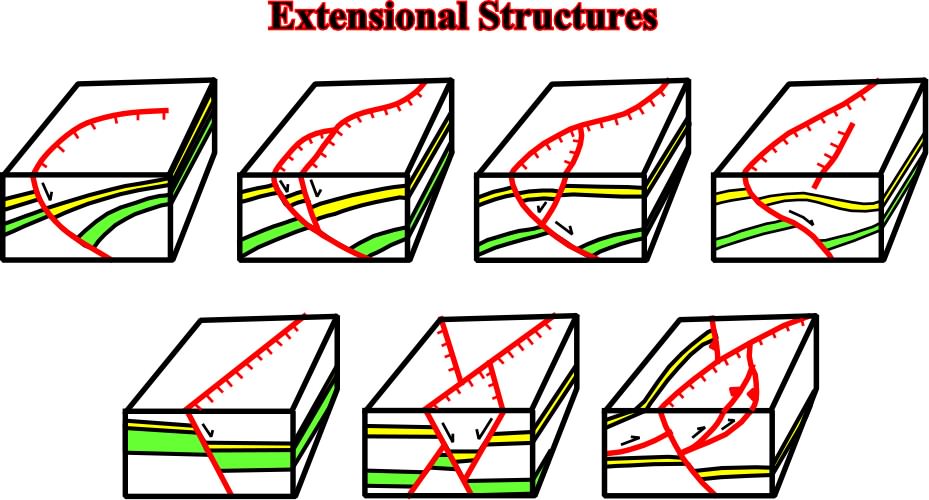
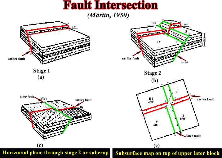
Flat topography: Fig. 112- The relationships between eroded surfaces, subcrop maps or seiscrops (all with flap topography) and the correlative cross-sections or seismic profiles are quite illustrated on these blocks diagrams. The geometry on the cross-sections or on seismic lines must match with the geometry on the flat surfaces. When a seismic interpreter recognizes a curvilinear normal fault on a seiscrop, the fault on a seismic profile must show, in depth, an increasing hade, i.e., its fault plane must flat in depth. Similarly, when two rectilinear normal faults intersect, on a flat surface, as well as on a cross-section, the youngest fault displaced the oldest. This hypothesis, which is only valid when the map (upper surface) is without or with a flat topography, is illustrated by two the lower right blocks.

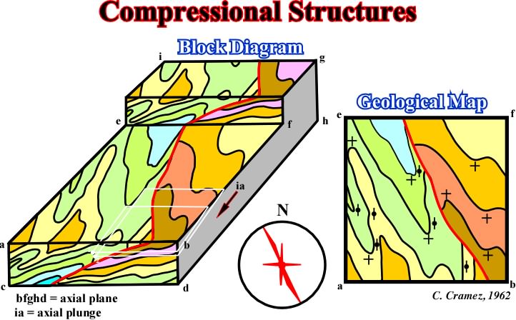
Fig. 113- The relationships observed in extensional structures (fig. 112) between horizontal surfaces (geological maps without topography, or seiscrops) and cross-sections (or seismic lines), must also be respected on compressional structures, particularly in those deformed by concentric folding. These relationships are summarized in this block diagram, in which the basic principles of 3D seismic interpretation are depicted. The strike of the more dipping beds gives roughly 2 (2= strike of vertical bed) and the dip of the less dipping beds gives the axial plunge. In other words, in an area with horizontal beds, the axial plunge of the structures is zero and the strike of the vertical beds is parallel to the axial plane of the structures (perpendicular to 3).

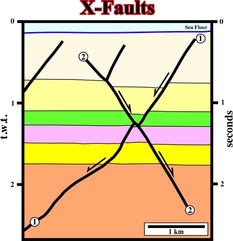
Fig. 114- This seismic line from Gulf of Mexico, illustrates a typical example of normal faults in X. The younger fault, dipping to the right, offsets the older on which dips to the left. In a seiscrop , or in a flat geological map, also the younger fault displaces the older one. However, as we will see below, in a time structural map or in a geological map with a significant topography, that is quite more complicated.

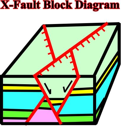
Fig. 115- In a cross-section ( or seismic line) the intersection of the normal faults X faults) are characterized by a graben structure overlying, in the same vertical, an horst structure., as illustrated on this block diagram and on the seismic line illustrated on fig. 114. The mapping of these faults depends on the level of cartography. In upper levels the mapping is relatively easy. We just need to make a dextral rotation of rotate 270� to get the geometry on the ground surface. However, as we will see in the next, the influence of the topography (see fig. 117) is quite important

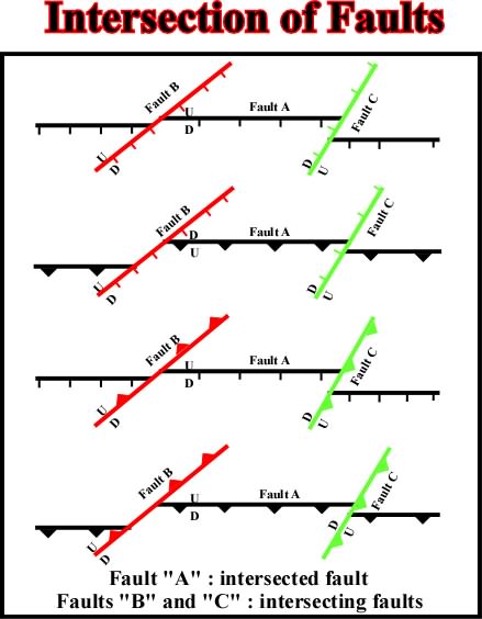
Fig. 116- This map illustrates various combinations of faults intersecting at different angles on a planar surface or on a non-conformity. The intersection of the intersected fault (in black) and the surface is invariably offset by the intersecting faults (red and green) in the direction of its dip in the upthrown block. This offset is independent of the intersection angle of the faults, providing the direction of movement of the intersecting fault is dip slip.

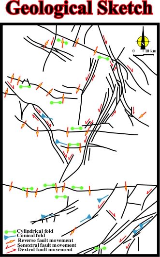
Fig. 117- On this geological sketch, it is evident that the sediments were shortened by compressional tectonic regime characterized by a 1 roughly North-South and a 3 vertical and/ or horizontal. All faults are contemporaneous. They were created by the same tectonic regime and so all them shortened the sediments, Subsequently, and contrariwise to the last extensional examples, the intersection relationships cannot be used to determined the relative age of the faults. Do not forget than in an extensional tectonic regime the faults are parallel to 2. If there are two fault systems striking in different directions, there are two consecutive extensional tectonic regimes with different 2.

Fig.118- Very often explorationists, when interpreting isochrone maps (time structural maps) do not take into account influence of the topography this possibility , i.e. time contour maps of deformed chronostratigraphic surfaces. In fact, on these maps, as a consequence of the topography, often younger faults are apparently offset by older faults.